Query Processing and Optimization

 

Query Cost Estimation

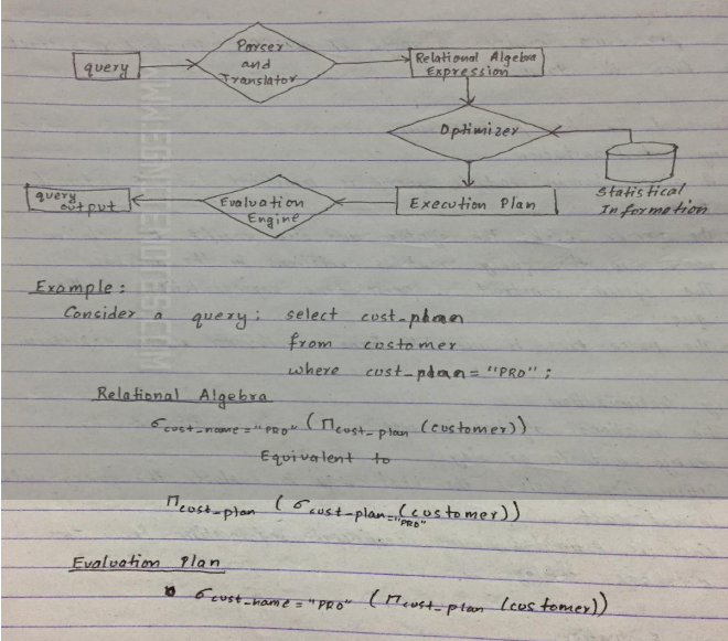
Query Processing

-Query processing involves a range of activities involved to extract data from database.

---

Steps involved in query processing

1) Parsing and Translation
a. A given human readable query is translated into its internal form.
b. The parser checks the syntax and also verifies the relation names in the query matches relations in database
c. The system construct a parse tree representation of the query.
d. The parse-tree is used to form a relational algebra expression

2) Query Optimization
a) The relational algebra expression can be evaluated by many methods or ways.
b) Optimization involves the best way to evaluate the query with lowest cost.
c) Cost is estimated using statistical information from the database catalog.

3) Query Evaluation
The evaluation engine takes a selected query evaluation plan, execute the plan and finally provides output to the users.

---

Query Cost Estimation

1) Cost is generally estimated as a response time for a query.
2) Response time depends on disk access, contents of buffer, network communication and so on.
3) Disk access is the predominant cost and is estimated by no of seeks, no of blocks read or written.
4) The cost for block transfer is :
5) A strategy is chosen based on statistical information for each relation that contains no of tuples, size of tuples and size if distinct values for a particular attribute.

---

Query Operation

Selection

- A1 (linear search)
Search each file block and test all records to determine satisfaction.
- A2 (Binary Search)
Selection is equality on attribute on which file is ordered.
- A3 (Primary index on candidate key , equality )
- A4 (primary index on non-key, equality.
- A5 (secondary index on search key, equality.
- A6 (primary index , comparison )
- A7 (secondary index, comparison )

---

Sorting:

- Quick sort (records completely in main memory )
- External sort ( records are on disk )

---

Join Operation

1. Nested loop join
- R ∞ S
- For each tuple t in r do begin
For each tuple ts in s do begin
Test pair (t, ts) to see if condition satisfy
If they do add t and ts to the result.
End
End

2. Merge loop join
- Sort both relations on their join attributes
- Used for natural joins

3. Hash join
- Used for natural join
- A hash function h is used to partition tuples of both relations

---

Evaluation of Expressions

Materialization:

- Executes a single operation at a time which generates a temporary file that will be used as ilp for next operation.
- It is easy to implement but time consuming.
- It walks the parse tree of relational algebra and perform innermost operations first.
- The result is materialized and becomes ilp for next operations.
- The cost is the sum of individual operations plus the cost of writing intermediate results to disks.
- It can always be applied.

---

Pipelining

- With pipeline, operations are arranged and form a queue and results are passed from one operation to another as they are calculated
- Avoids intermediate temporary relations.
- Cheaper as no cost of writing results to disk
- It is not always possible.
- In demand driven system requests next tuple from top level operation, each operation requests next tuple from children operation.
- In producer driven, operators produce tuples and pass to parents.

---

Query Optimization

- It is the process of selecting most efficient query evaluation plan.
- At relational algebra level, the system attempts to find an expression equivalent to given one but is more efficient.
- An algorithm can be chosen.

---

Transformation of relational expressions

- Two relational algebra expressions are said to be equivalent if, one or every legal database instance both expressions generate the same set of tuples.
- This is the first step of optimization,
- It generates logically equivalent expressions to the given expressions using equivalence rules.

---

Equivalence Rules

1. Conjunctive selection operations can be deconstructed into a
sequence of individual selections.
σθ1^θ2(E) = σθ1(σθ2(E))

2. Selection operations are commutative.
σθ1(σθ2(E)) = σθ2(σθ1(E))

3. Only the last in a sequence of projection operations is
needed, the others can be omitted.
Πt1 ( Πt2 (.... (Πtn (E)))) = Πt1 (E)

4. Selections can be combined with Cartesian products and
theta joins.
a. σθ(E1 X E2) = E1 ⋈θ E2
b. σθ1(E1 ⋈θ2 E2) = E1 ⋈θ1∧ θ2 E2

5. Theta-join operations (and natural joins) are commutative.
E1 ⋈θ E2 = E2 ⋈θ E1

6. (a) Natural join operations are associative:
(E1 ⋈ E2) ⋈ E3 = E1 ⋈ (E2 ⋈ E3)

(b) Theta joins are associative in the following manner:
(E1 ⋈θ1 E2) ⋈θ2∧ θ 3 E3 = E1 ⋈θ1∧ θ3 (E2 ⋈θ2 E3)
where θ2 involves attributes from only E2 and E3.

7. The selection operation distributes over the theta join operation
under the following two conditions:
(a) When all the attributes in θ0 involve only the attributes of one
of the expressions (E1) being joined.
σ ⋈θ0(E1 ⋈θ E2) = (σ ⋈θ0 (E1)) ⋈θ E2

(b) When θ 1 involves only the attributes of E1 and θ2 involves
only the attributes of E2.
σθ1∧θ2 (E1 ⋈θ E2) = (σθ1(E1)) ⋈θ (σθ2 (E2))

8. The projections operation distributes over the theta join operation
as follows:
(a) if Π involves only attributes from L1 ∪ L2:
ΠL1∪L2 (E1 ⋈θ E2) = (ΠL1(E1)) ⋈θ (ΠL2(E2))

(b) Consider a join E1 ⋈θ E2.
- Let L1 and L2 be sets of attributes from E1 and E2, respectively.
- Let L3 be attributes of E1 that are involved in join condition θ, but are not in L1 ∪ L2, and
- let L4 be attributes of E2 that are involved in join condition θ, but are not in L1 ∪ L2.
ΠL1∪L2 (E1 ⋈θ E2) = ΠL1∪L2((ΠL1∪L3(E1)) ⋈θ (ΠL2∪L4(E2)))

9. The set operations union and intersection are commutative
E1 ∪ E2 = E2 ∪ E1
E1 ∩ E2 = E2 ∩ E1
! (set difference is not commutative).

10. Set union and intersection are associative.
(E1 ∪ E2) ∪ E3 = E1 ∪ (E2 ∪ E3)
(E1 ∩ E2) ∩ E3 = E1 ∩ (E2 ∩ E3)

11. The selection operation distributes over ∪, ∩ and –.
σθ (E1 – E2) = σθ (E1) – σθ(E2)
and similarly for ∪ and ∩ in place of –
Also: σθ (E1 – E2) = σθ(E1) – E2
and similarly for ∩ in place of –, but not for ∪

12. The projection operation distributes over union
ΠL(E1 ∪ E2) = (ΠL(E1)) ∪ (ΠL(E2))

---

Choice of Evaluation plan

1) Cost based optimization
a. It explores the space of all query evaluation plans that are equivalent to given query and chooses one with least estimated cost.
b. Exploring space of all possible plans may be expensive.
c. It guarantees finding of optimal plans.

2) Heuristic optimization
a. System uses heuristics to reduce number of choices to evaluate,
b. A query is transformed by using a set of rules as:
i. Perform selection early
ii. Perform projection early
iii. Perform most restrictive selection and join operations before other similar operations.

---

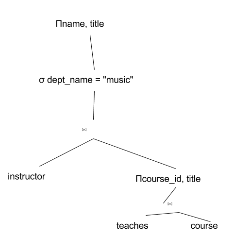
Optimize the query: Πname, title (σ dept_name = "music" (instructor ⋈ Πcourse_id, title (teaches ⋈ course)))

The initial expression tree is given below:

---

Using ΠL (E1 ⋈ E2) = E1 ⋈ ΠL (E2), we get:
Πname, title (σ dept_name = "music" (instructor ⋈ (teaches ⋈ Πcourse_id, title(course))))

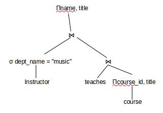
Using σL (E1 ⋈ E2) = σL (E1) ⋈ E2, we get:
Πname, title (σ dept_name = "music" (instructor) ⋈ (teaches ⋈ Πcourse_id, title(course)))

---

Query Decomposition

- It transforms SQL query into relational algebra query.
- The steps involved are as follows:
1. Normalization
2. Analysis
3. Redundancy Elimination
4. Rewriting