Control System

 

Open Loop and Closed Loop Control System

Control System

Control system is a system designed to control physical system output to a desired limit by setting desired reference output.

-Automobile Cruise Controller
This controller seeks to make a car’s speed track a desired speed by setting the car’s throttle and brake inputs by setting the car’s throttle and brake inputs.

-Thermostat controller
It forces a building temperature to a desired temperature by turning on the heater or Air Conditioning System and adjusting the fan speed.

---

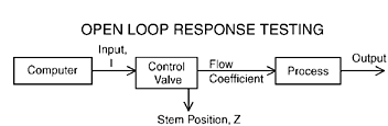
Open Loop Control System

- It is a feed forward control system

-It consists of following parts:

1. Plant process
-It is the physical system to be controlled.

2. Output
-It is the particular aspect of physical system that we intend to control.

3. Reference input
-It is the desired value that we want to see for the output.

4. Actuator
-It is the device used to control i/p to the plant.

5. Controller
-It is the system used to compute the i/p to the plant.

6. Disturbance
-It is an additional undesirable i/p imposed by environment that causes o/p to differ from out expectation.

---

Designing Open Loop control system

Model of plant
Model of the plant is developed to make design phase easier and to desire the controller. For ex Throttler
That goes from 0 to 45 degrees.
-On flat surface at 50 mph ,open throttle to 40 degree.
-Wait 1 “time unit"
-Measure the speed , lets say 55 mph
-Then the equation that holds for all scenarios gives model of the plant.

v(t+1) = 0.7 v(t) + 0.5 u(t)
55 = 0.7 * 50 + 0.5 * 40

 

Controller design
Controller provides a specific rule to achieve the goal of the control system.

Assume we have a linear function:
U(t) = F[r(t)] = P*r(t) 
                      where, P = constant , 
                                   r(t)  = desired speed..
Now, 
           v(t+1)  = 0.7*v(t)  + 0.5*u(t)  =  0.7*v(t) + 0.5*P*r(t) 

 

Let v(t+1) = v(t); at steady state = v(ss) ;
v(ss) = 0.7*v(ss) + 0.5*P*r(t)

At steady state we want v(ss) = r(t)

1= 0.7+0.5*P
P = 0.6

Hence the control rule is defined as:
u(t) = P*r(t) = 0.6* r(t)

 

Analyzing Controller

Suppose,
 v(0)  = 20mph and r(0)  = 50mph 

 

Then , vt+1 = 0.7 *v(t) + 0.5*0.6*r(t)
=0.7*v(t) + 0.3*50
=0.7*v(t) + 15

Therefore throttle position = 0.6*50 = 30 degree

 

Considering Disturbance

Assuming road grade affect speed from -5mph to +5 mph

 

Time v(t) v(t) [w = +5] v(t) [w = -5]
0 20 20 20
1 29 24 34
2 35.3 26.80 43.80
3 39.71 28.76 50.66
4 42.80 30.13 55.46
5 44.96 31.09 58.82
6 46.47 31.76 61.18
7 47.53 32.24 62.82
8 48.27 32.56 63.98
9 48.79 32.80 64.78
10 49.15 32.96 65.35
11 49.41 33.07 65.74
12 49.58 33.15 66.02

 

Determining performance

     v(t+1) =  0.7*v(t)  + 0.5*u(t)   - w(0)
     v(1) = 0.7*v(0)  + 0.5*u(0)   - w(0)
      v(2)  = 0.7(0.7*v(0)  + 0.5*u(0)   - w(0)) + 0.5P * r(0) – w(0)
      v(t)  =0.72v(0) + ( 0.7^(t-1) + 0.7^(t-2)+ ……….. +0.7 + 1)(0.5P*r(0) – w(0))

- Coefficient of v(t) determines rate of decay of v(0)
- If > 1 or < -1 , v(t) will grow without bound
- Otherwise v(t) will oscillate.

 

---

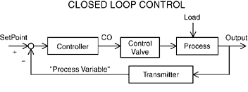
Closed Loop Control System

-It is a feedback control system.
-It minimizes tracking error.
-It consists of some additional part (sensors to measure plant o/p and error detector to detect errors and mistakes in the data).

---

Designing Closed Loop Control System

Design model of plant

     v(t+1) =  0.7*v(t)  + 0.5*u(t)   - w(t)

 

Design Controller

 
     U(t)  =  P(r(t)  - v(t) )

 

v(t+1) = 0.7*v(t) + 0.5 P(r(t) - v(t)) - w(t)
= (0.7- 0.5P)v(t) + 0.5P * r(t) - w(t)

v(t) = (0.7- 0.5P)^t * v(0) + { (0.7- 0.5P)^(t-1) + (0.7- 0.5P)^(t-2) + …… + (0.7- 0.5P) +1 } ( 0.5 P * r(0) - w(0))

So,
Stability constraint requires:
|0.7 – 0.5P| <1
Or, -1< 0.7 -0.5P <1
Thus, -0.6

 

 

Reducing effect of v0
To reduce the effect of initial condition (i.e. v0) ,
a) 0.7 – 0.5p must be as small as possible.
i.e. 0.7-0.5p = 0 ;
thus, p = 1.4

Avoid Oscillation
To avoid oscillation, 0.7-0.5p must be greater than or equal to 0.
i.e. 0.7 – 0.5p >= 0
therefore, p<=1.4

Perfect Tracking

Assume at steady state v(ss)  , v(t+1)  = v(t)  ;

 

V(ss) = (0.7 -0.5p)v(ss) + 0.5 P * r(0) – w(0)
Or (1-0.7+0.5p)v(ss) = 0.5 P * r(0) - w(0)
So, v(ss) = (0.5 P * r(0) - w(0)) / (0.3+ 0.5p)
= 0.5 / (0.5 P * r(0) - w(0)) * r(0) - 1 / (0.3+ 0.5p) * w0

To make vss close to r0 ­ , p should be as large as possible.

 

Analyse controller
-set P=3.3 , saturate at 0.45, oscillation
-set p=1 to avoid oscillation . Terrible SS performance.

---

Control System and PID Controller

P controller

- It multiplies the tracking error by a constant.
- u(t) = P[r(t) – v(t)]
- P affects transient response (stability ),steady state tracking error and disturbance rejection .

---

PD controller

- It considers the size of error over time.
- It keeps track of error derivative.
- u(t) = P*e(t) + delta*[e(t) – e(t-1))
- P set for best tracking and disturbance control.
- D set to control oscillation and convergence rate

---

PI controller

- It sum up error over time.
- u(t) =P*e(t) + I* (e(0) + e(1) + …… + e(t))
- P controls disturbance.
- I ensures steady state convergence.

---

PID Controller

- Combines proportional , integral and derivative control.
- u(t) = P*e(t) + delta*[e(t) – e(t-1)) + I* (e(0) + e(1) + …… + e(t))
- It achieves desired stable transient behavior.

---

The block diagram of PID Controller is shown below:

---

Software Coding of a PID Controller

Code in C:

 

//Sample Coding for PID controller

 

..including different library files..

void main() {
double sen_val,act_val,err_current;
PID_DATA pid_data;
PidInitialize(&pid_data);
while(1)
{
sen_val = SensorGetValue();
ref_val= ReferenceGetValue();
act_val = PidUpdate(&pid_data,sen_value,ref_val);
ActuatorSetValue(act_value);
}

}

typedef struct PID_DATA {
double Pgain,Dgain,Igain ;
double sen_val_previous ; //Find derivative
double error_sum ; //cumulative error
}

//definition of function PidUpdate
double PidUpdate(PID_DATA * pid_data , double sen_val,double ref_val)
{
double Pterm,Iterm,Dterm;
double err,diff;
err = ref_val – sen_val ;
Pterm =pid_data->Pgain* err;
pid_data ->error_sum+= error;
Iterm =pid_data ->Igain*pid_data->error_sum ;
diff=pid_data->sen_val_previous = sen_val;
Oterm = pid_data ->Dgain* diff;
return (Pterm + Iterm+Dterm);
}

 

---

PID Tuning

-Pid tuning is the process of obtaining P,I and delta by ad-hoc methods.
-It is necessary because:
a) with analytics , the plant model may be complex .
b) we may not even have a plant model

---

Algorithm for PID Tuning:

1. Start with a small P, I=D=0

2. Increase D until seeing oscillation
-Decrease delta a bit

3. Increase P until seeing oscillation
-Decrease P a bit

4. Increase I, until seeing oscillation

5. Repeat from second step until performance can be improved.

---

Issues with computer based control

1)Quantization and overflow

-quantization occurs when a signal must be altered to fit memory constraints.
-arithmetic operations cause quantization.
-e,g, assume an operation results 0.36 but it must be stored as 4 bit fractional number , so 0.25 is choosed instead of 0.36
-Overflow occurs when operation outputs a number with magnitude too large to be represented by a processor and thus chances of error.
-Uses fixed point representation carefully(time consuming)
-Uses floating point and co-processor(expensive)

2)Aliasing

-Aliasing is due to the discrete nature of sampling.
- Example : Sampling at 2.5 Hz, period of 0.4;
y(t) = 1.0 * sin (6 * pi * t), f = 3Hz
y(t) = 1.0 * sin (pi * t), f = 0.5Hz
These two functions are indistinguishable.

3) Computational Delay

- The computation causes delay to occur that causes actuation to delay.
- The implementation delay must be negligible.
- Software delay is hard to predict.

---

Benefits of Computer Based Control

1. Cost
2. Programmable
3. Reproducible

---