Analysis of simulation output

 

Estimation methods

Simulation Output : Introduction

- Whenever a random variable is introduced to the simulation model, all the system variables that describe its behaviour become random or stochastic.
- The values of the variables involved in the system will fluctuate as the simulation proceeds.
- So, arbitrary measurement of the values of these variables can not represent the true value.
- For this, some conditions about the probability of the true value falling within a given interval about the estimated value must be made. Such interval is known as confidence interval.
- In simulation study, it is assumed that the observations being made are mutually independent. But, in most of the real world problems, simulation results are mutually dependent.
- The various methods used to analyze simulation results are as follows:
1. Estimation Methods
2. Simulation Run Statistics
3. Replication of Runs
4. Elimination of Initial Bias

---

Estimation Method

- It is assumed that the random variables are stationary and independent drawn from an infinite population with a finite mean and finite variance.
- Such random variables are independently and identically distributed (IID) random variable.
- The central limit theorem can be applied to IID data. It states that “the sum of n numbers of IID variables, drawn from a population that has a mean of μ and a variance of σ², is approximately distributed as a normal variable with a mean of nμ and a variance of nσ².”
- The normal distribution can be transformed into a standard normal distribution, that has a mean of 0 and a variance of 1.

---

Example:

Let us consider x(i) where i = 1, 2, 3, …………, n be the n number of random variables drawn from a sample of population with mean μ and variance σ^2.
Using central limit theorem, and transforming to standard normal distribution, we get:

Z = (∑ x(i) - nμ) / {n^(½) * σ}

Dividing top and bottom by n, we get:

Z = ( x - μ) / (σ / n^(½))
Where x = ∑ x(i) / n = sample mean

---

Confidence Interval Estimation

- The sample mean acts as a consistent estimator for the mean of population from which the sample is drawn; which is also a random variable.
- As sample mean is random, confidence interval about its computed value should be established.
- The probability density function of the standard normal variate is shown in given figure:

---

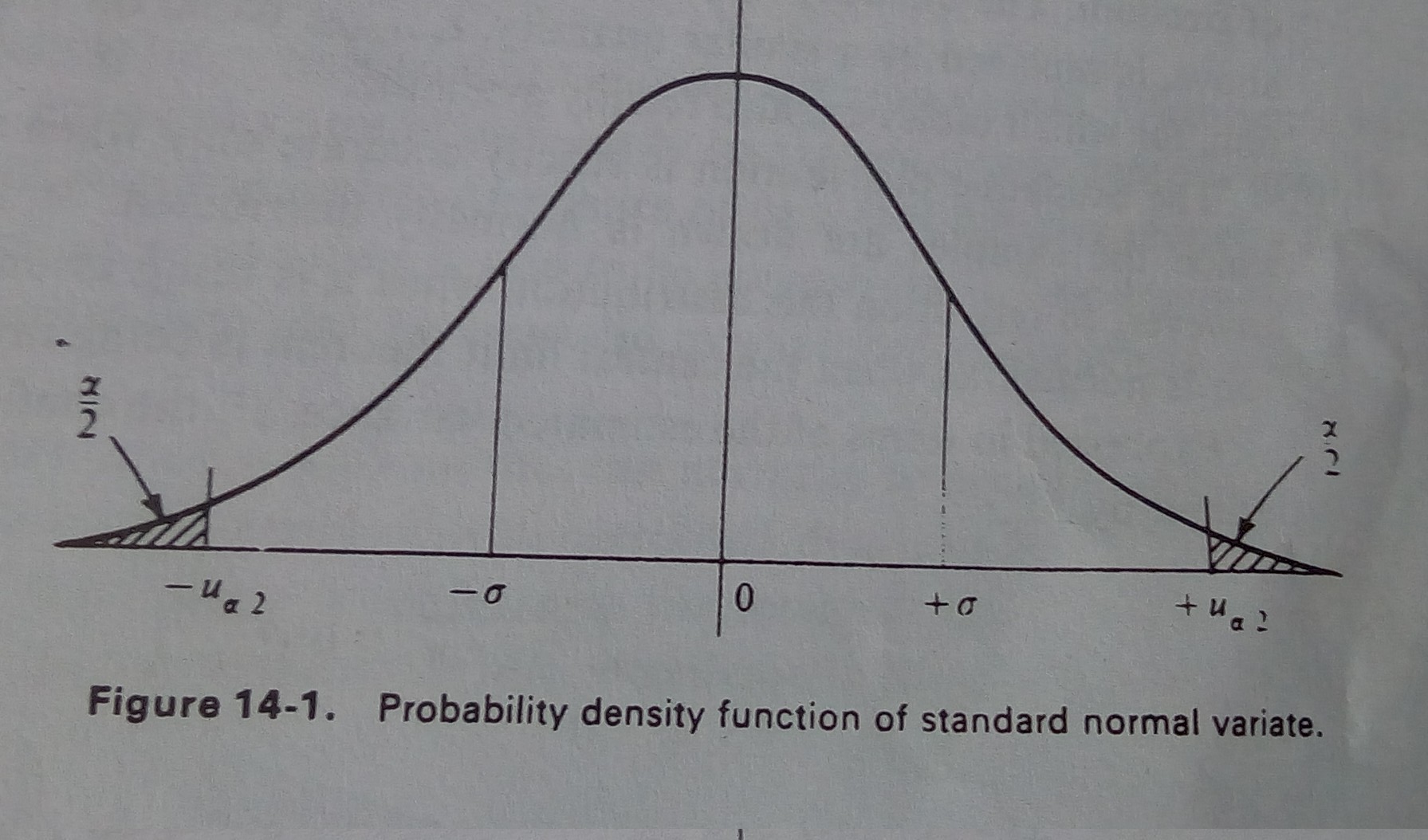
- For some constant α, known as level of significance, the probability that z lies between -u(α/2) and u(α/2) is given by:

P( - u(α/2) <= z <= u(α/2) ) = 1 - α

Putting the value of z from point estimation, we get:

P( - u(α/2) <= ( x - μ) / (σ / n^(½)) <= u(α/2) ) = 1 - α
P( - u(α/2) * (σ / n^(½)) <= ( x - μ) <= u(α/2) * (σ / n^(½)) ) = 1 - α
P( u(α/2) * (σ / n^(½)) + x >= (μ) >= - u(α/2) * (σ / n^(½)) + x ) = 1 - α

Hence, the confidence interval is given by:

X (+ or -) u(α/2) * (σ / n^(½))

---

Simulation run statistics

- In most of the simulation study, the assumptions of stationary and mutually independent observations do not apply. An example of such case is queuing system.
- Correlation is necessary to analyze such scenario.
- In such cases, simulation run statistics method is used.

---

Example:

- Consider a system with Kendall’s notation M/M/1/FIFO and the objective is to measure the mean waiting time.
- In simulation run approach, the mean waiting time is estimated by accumulating the waiting time of n successive entities and then it is divided by n. This measures the sample mean such that:

x = ∑ x(i) / n for i = 1 to n

- Such series of data in which one value affect other values is said to be autocorrelated.
- The sample mean of autocorrelated data can be shown to approximate a normal distribution as the sample size increases.

---

Problem:

- The distribution may not be stationary.
- A simulation run is started with the system in some initial idle state.
- In this case, the early arrivals will obtain service quickly deviating from normal distribution.
- Hence, the sample means of the early arrivals is known as initial bias.
- As the sample size increases and the length of run is long, the effect of bias dies and the normal distribution is again established.

---

Replication of runs

- This approach is used to obtain independent results by repeating the simulation.
- Repeating the experiment with different random numbers for the same sample size n gives a set of independent determinations of the sample mean x(n).
- The mean of the means and the mean of the variances are then used to estimate the confidence interval.
- Consider that the experiment is repeated p times over the n random variables.
- Let x(i,j) represents jth random variables on ith simulation run.
- We can write:

x = ∑ x(j) / p for j = 1 to p

Where,
x(j) = ∑ x(j,i) / n for i = 1 to n

- The variance can be given by:

d^2 = ∑ d(j)^2 / p for j = 1 to p

Where,
d(j)^2 = ∑ {x(j,i) - x(j)} / (n-1) for i = 1 to n

---

Elimination of Initial bias

- The ways to eliminate the initial bias are as follows:
1. Ignore the initial bias occured during the simulation run.
2. The system should be started in a representative state than in the empty state.
3. Start the simulation in the empty state, then stop after initial bias and then start again.
4. Run the simulation for such a long period of time so that the initial bias has no any significance in the output result.